Correlation
If we want to examine the relationship between two continuous variables then calculate the correlation coefficient commonly known as Pearson’s r. The correlation coefficient ranges from \(-1\) to \(1\) where \(-1\) indicates a perfect negative relationship between the two variables and \(1\) a perfect positive relationship.
We calculate the correlation coefficient by using the cor() function.
For example, load the EVS_UK dataset. We will examine the relationship between peoples’ attitudes towards EU (v198) and attitudes towards immigration (v185). The interpretation of the results depends upon the direction of the values. In our case our two continuous variables range from \(0\) to \(10\), for v198 \(0\) means that the responder is against the enlargement of the EU and 10 in favour. For v185, \(0\) means that the responder believe that immigrants do not take away jobs while \(10\) means that they do take jobs away.
load("EVS_UK.RData")
cor(y=EVS_UK$v198, x=EVS_UK$v185, use="complete.obs")
## [1] -0.2465359Our coefficient is equal to \(-0.24\), the \(-\) sign indicates that there is a negative correlation between the two variables. A negative correlation means that there is an inverse relationship between two variables - when one variable decreases, the other increases. In other words, higher values of one variable tend to be associated with lower values of the second variable.
The opposite is a positive correlation, when one variable decreases as the other variable decreases, or one variable increases while the other increases.
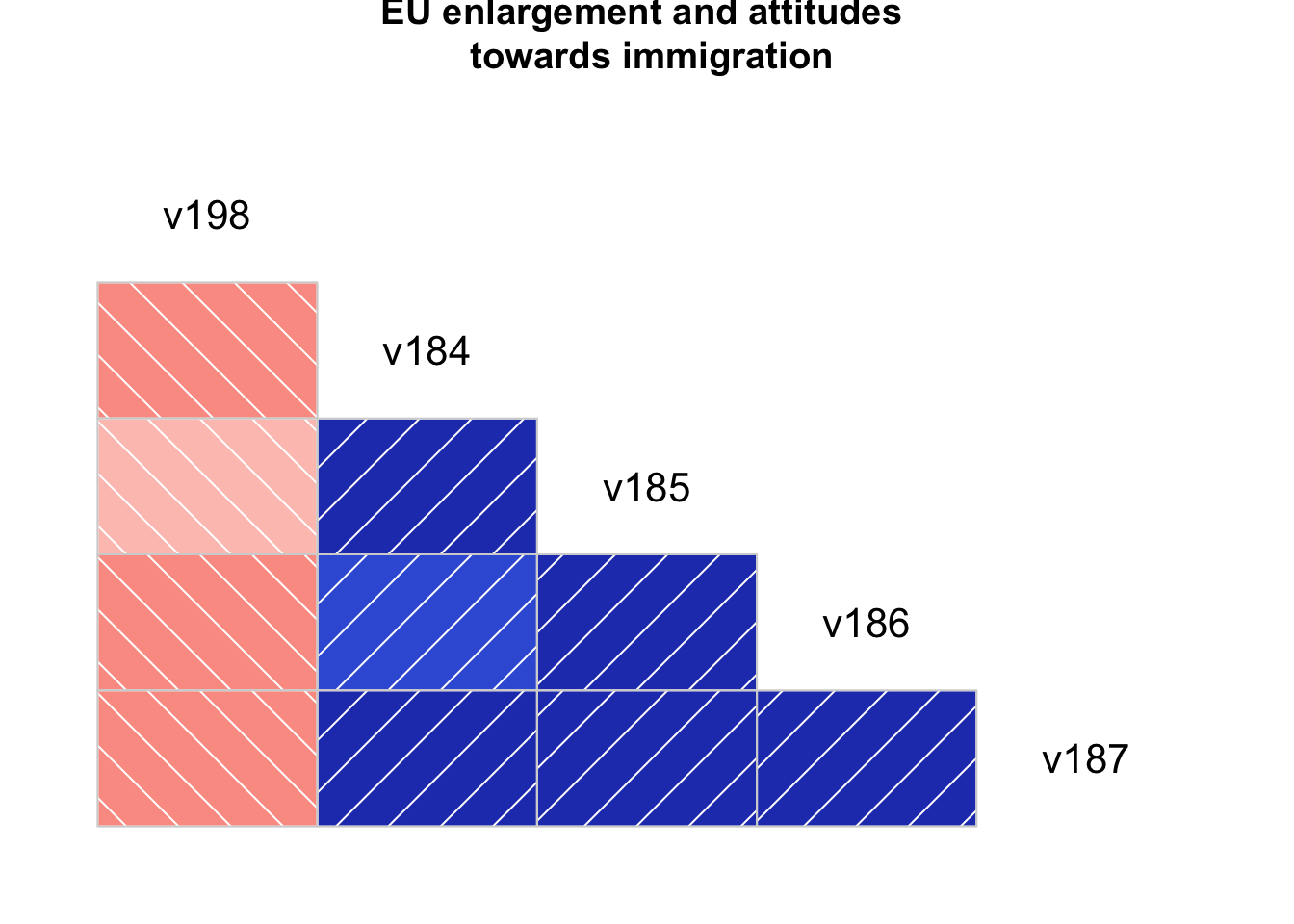
You may visualise the relationship between two variables by creating a correlogram:
We start by creating a subset of our dataset, our subset will include the two variables we are interested in, v198 and v185, and few more variables measuring attitudes towards immigration v184, v186, and v187.
evs_subset <- c("v198", "v184", "v185", "v186", "v187")
euimmi.sample <- EVS_UK[evs_subset]
View(euimmi.sample)
let’s confirm that all of our variables are numeric i.e. continuous
class(EVS_UK$v198)## [1] "haven_labelled"class(EVS_UK$v185)## [1] "haven_labelled"class(EVS_UK$v186)## [1] "haven_labelled"class(EVS_UK$v187)## [1] "haven_labelled"EVS_UK$v198<-as.numeric(EVS_UK$v198)
EVS_UK$v185<-as.numeric(EVS_UK$v185)
EVS_UK$v186<-as.numeric(EVS_UK$v186)
EVS_UK$v187<-as.numeric(EVS_UK$v187)Visualising correlations
Don’t forget to install the package we will use by using the install.packages() function:
install.packages("corrgram")
library(corrgram)
corrgram(euimmi.sample, order=NULL, lower.panel=panel.shade,
  upper.panel=NULL, text.panel=panel.txt,
  main="EU enlargement and attitudes \n towards immigration")