The model
We are now ready to conduct our analysis. We will use the lm() function.
library(lme4)
model.1<-lm(immi.jobs~ born.country+respect.inst+country.ancestry+speak.lang+share.cultr+left_right+education+gender+age,data=sub.sample)
summary(model.1)
##
## Call:
## lm(formula = immi.jobs ~ born.country + respect.inst + country.ancestry +
## speak.lang + share.cultr + left_right + education + gender +
## age, data = sub.sample)
##
## Residuals:
## Min 1Q Median 3Q Max
## -6.1341 -1.6810 -0.1593 1.6917 7.8835
##
## Coefficients:
## Estimate Std. Error t value Pr(>|t|)
## (Intercept) 1.2363291 0.4307600 2.870 0.004157 **
## born.country 0.5846284 0.0780512 7.490 1.13e-13 ***
## respect.inst -0.0589700 0.1056487 -0.558 0.576805
## country.ancestry 0.4367903 0.0854104 5.114 3.53e-07 ***
## speak.lang 0.3575283 0.1150266 3.108 0.001915 **
## share.cultr 0.3870998 0.1052285 3.679 0.000242 ***
## left_right 0.0354641 0.0313352 1.132 0.257901
## education -0.0017546 0.0002726 -6.436 1.62e-10 ***
## gender -0.3156420 0.1180030 -2.675 0.007551 **
## age 0.0014324 0.0036699 0.390 0.696364
## ---
## Signif. codes: 0 '***' 0.001 '**' 0.01 '*' 0.05 '.' 0.1 ' ' 1
##
## Residual standard error: 2.355 on 1614 degrees of freedom
## (164 observations deleted due to missingness)
## Multiple R-squared: 0.2354, Adjusted R-squared: 0.2311
## F-statistic: 55.21 on 9 and 1614 DF, p-value: < 2.2e-16library(dotwhisker)dwplot(list(model.1), vline = geom_vline(xintercept = 0, colour = "grey60", linetype = 2)) %>% # plot line at zero _behind_ coefs
relabel_predictors(c(immi.jobs = "Immigrants take jobs",
born.country = "Born in country",
respect.inst = "Respect institutions",
country.ancestry = "Country ancestry",
speak.lang = "Speak language",
share.cultr = "Share culture",
left_right="Left-Right",
education="Education",
gender="Gender",
age="Age")) +
theme_classic() + xlab("Coefficient Estimate") + ylab("") +
geom_vline(xintercept = 0, colour = "grey60", linetype = 2) +
ggtitle("Predicting anti-immigration attitudes") +
theme(plot.title = element_text(face="bold"),
legend.position = c(0.01, 0.03),
legend.justification = c(0, 0),
legend.background = element_rect(colour="grey80"),
legend.title = element_blank()) 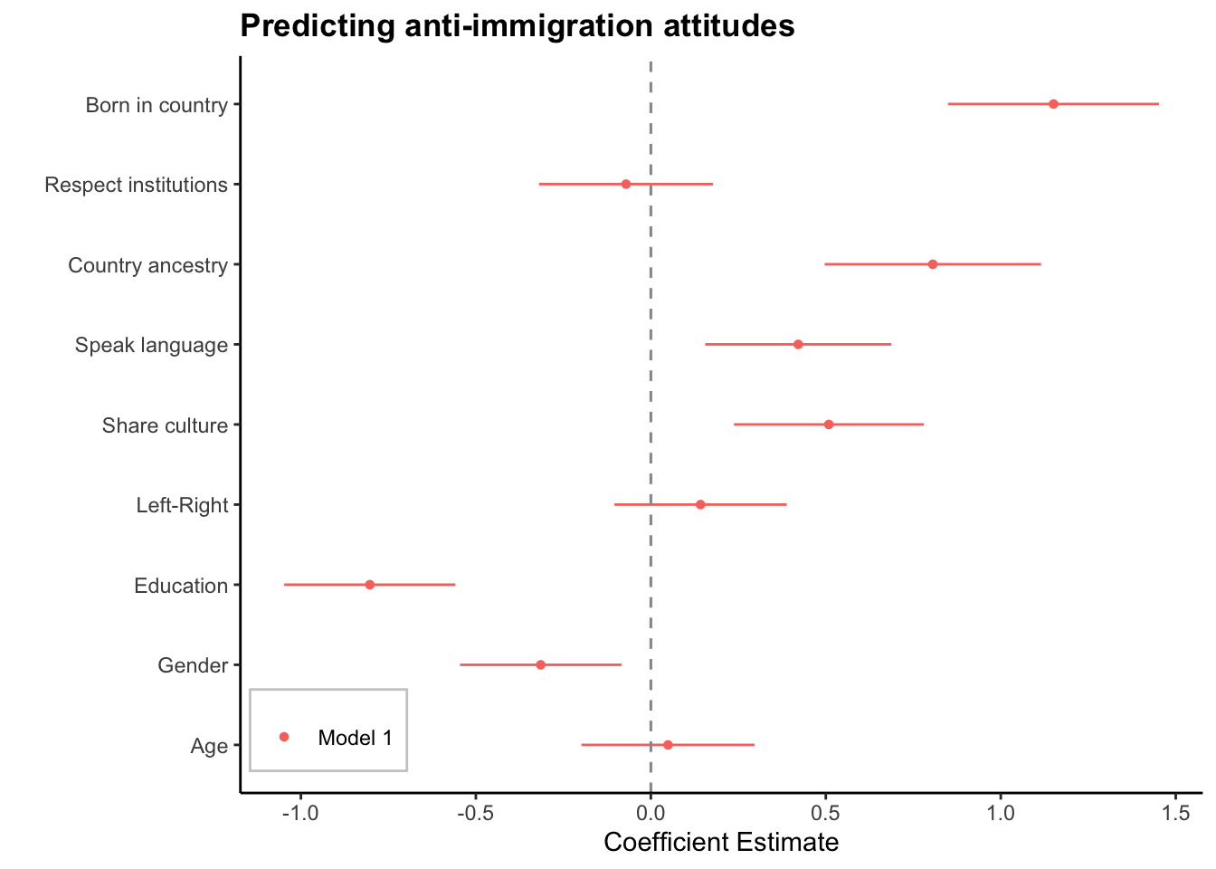
From our analysis we can see that three of our variables are not statistically significant, namely age, respect towards institutions, and left-right. Let’s construct another model but this time we will exclude the three variables that are not statistically significant.
model.2<-lm(immi.jobs~ born.country+country.ancestry+speak.lang+share.cultr+education+gender,data=sub.sample)
summary(model.2)
##
## Call:
## lm(formula = immi.jobs ~ born.country + country.ancestry + speak.lang +
## share.cultr + education + gender, data = sub.sample)
##
## Residuals:
## Min 1Q Median 3Q Max
## -6.2424 -1.7014 -0.1612 1.7130 7.7064
##
## Coefficients:
## Estimate Std. Error t value Pr(>|t|)
## (Intercept) 1.274658 0.356722 3.573 0.000362 ***
## born.country 0.581489 0.075558 7.696 2.34e-14 ***
## country.ancestry 0.502525 0.082420 6.097 1.33e-09 ***
## speak.lang 0.350976 0.109172 3.215 0.001329 **
## share.cultr 0.381239 0.098778 3.860 0.000118 ***
## education -0.001789 0.000258 -6.932 5.80e-12 ***
## gender -0.278855 0.114744 -2.430 0.015189 *
## ---
## Signif. codes: 0 '***' 0.001 '**' 0.01 '*' 0.05 '.' 0.1 ' ' 1
##
## Residual standard error: 2.377 on 1742 degrees of freedom
## (39 observations deleted due to missingness)
## Multiple R-squared: 0.2364, Adjusted R-squared: 0.2338
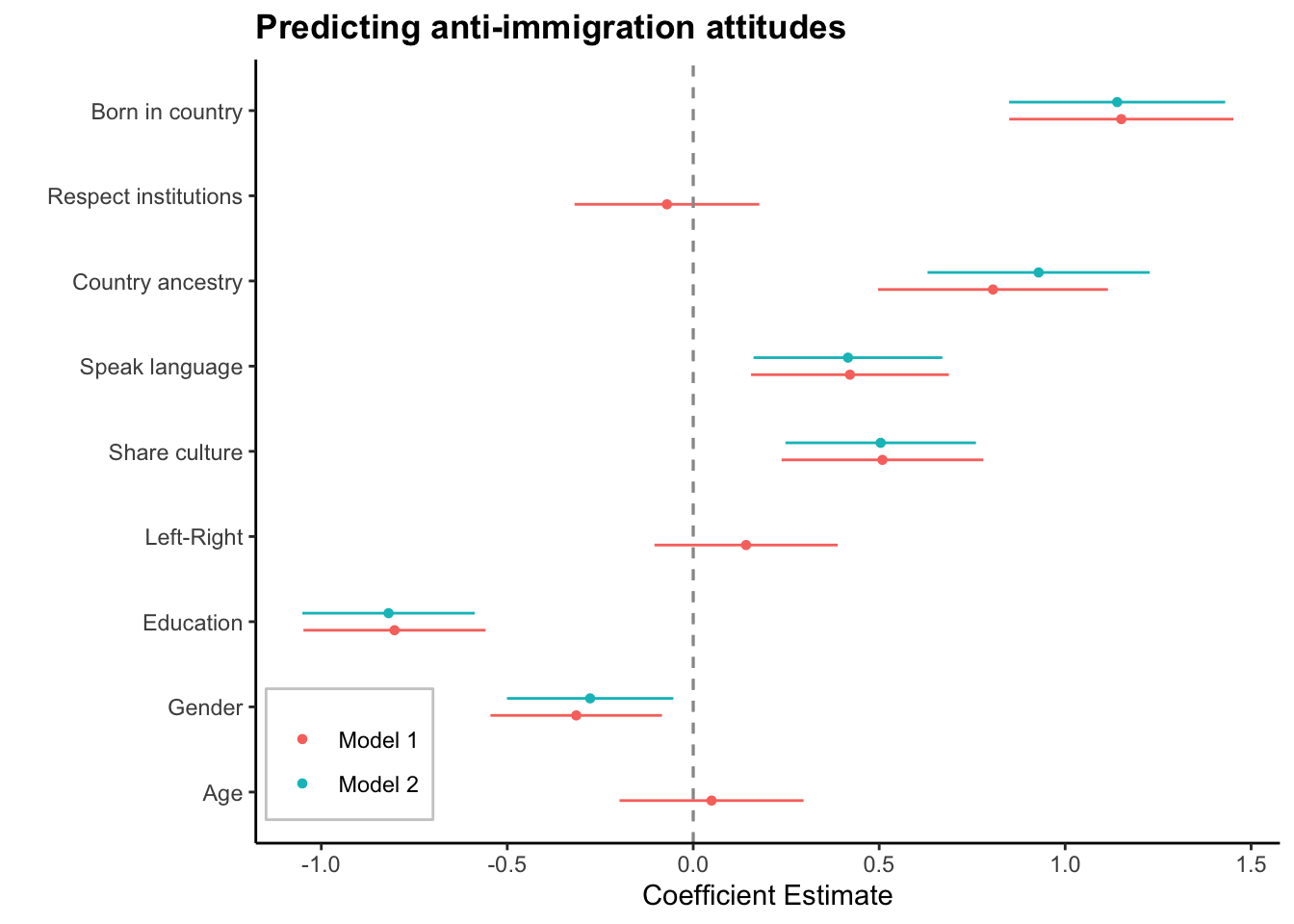
## F-statistic: 89.88 on 6 and 1742 DF, p-value: < 2.2e-16We can now plot both models and compare the results.
dwplot(list(model.1, model.2), vline = geom_vline(xintercept = 0, colour = "grey60", linetype = 2)) %>% # plot line at zero _behind_ coefs
    relabel_predictors(c(immi.jobs = "Immigrants take jobs",
                         born.country = "Born in country",
                         respect.inst = "Respect institutions",
                         country.ancestry = "Country ancestry",
                         speak.lang = "Speak language",
                         share.cultr = "Share culture",
                         left_right="Left-Right",
                         education="Education",
                         gender="Gender",
                         age="Age")) +
     theme_classic() + xlab("Coefficient Estimate") + ylab("") +
     geom_vline(xintercept = 0, colour = "grey60", linetype = 2) +
     ggtitle("Predicting anti-immigration attitudes") +
     theme(plot.title = element_text(face="bold"),
           legend.position = c(0.01, 0.03),
           legend.justification = c(0, 0),
           legend.background = element_rect(colour="grey80"),
           legend.title = element_blank())